Google Spreadsheets tips – For office work like number-crunching, invoices, spreadsheets, graphs, etc., Microsoft Office is the software to do it. However, thanks to the cloud, Google Docs is becoming popular day by day. In fact, Google Spreadsheets is becoming the choice for many users who use Excel. The good thing about Google Spreadsheets is that it is very simple to use, free and is as powerful as Microsoft Excel.
That being said, here are some of the best Google Spreadsheet tips that every Google Sheets user should know to get most out of Google Docs.
Google Spreadsheets Tips
1. Freeze Rows and Columns
When working on a spreadsheet, you might want to display certain columns and rows always on the screen. For instance, when you have the data like serial numbers and months, you might want to display those columns and rows so that you won’t lose track of them even while you are scrolling.
To freeze rows, select the first cell on the line, select the option “View > Freeze” and then select the option “1 row” to freeze the first row and “2 rows” to freeze the first two rows.
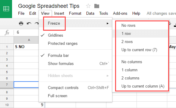
If you want to freeze more than two rows then select the cell as required and then select the option “Up to current row.” You can also freeze columns in the same way.
2. Quickly Insert Image Into a Cell
Generally, you can insert any image you want by simply selecting the option “Insert > Image.” When you use this option, the image will appear on top of the cells in the spreadsheet.
As you can tell, the above option is useless if you want to insert an image into a cell. To insert an image into a cell, select the cell and use one of the below functions.
=image("URL of the image",1)– resizes the image to fit inside the cell, maintaining aspect ratio. This is the default option when you use the =image formula without the mode(1, 2, 3) option.=image("URL of the image",2)– stretches or compresses the image to fit inside the cell, ignoring aspect ratio.=image("URL of the image",3)– leaves the image at original size, which may cause cropping.
3. List All Keyboard Shortcuts
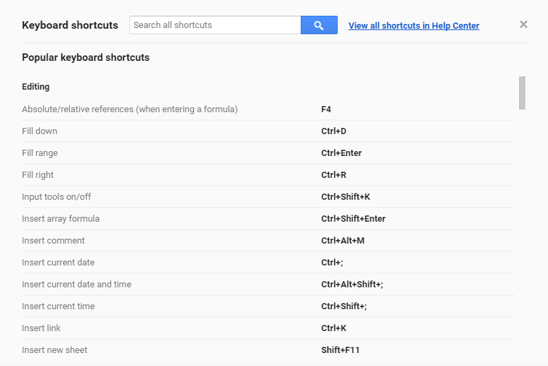
Keyboard shortcuts help us to do a lot of things without the need for using your mouse. That being said, it is not that easy to remember all the Google Sheets keyboard shortcuts all the time.
To see all the available keyboard shortcuts, simply press the below keyboard shortcut
Ctrl + /– for Windows.Command + /– for Mac.
Remember this single keyboard shortcut and you know all the Google Sheets keyboard shortcuts.
4. Create QR Codes
QR codes make is very easy to share data like big URLs, contact details, addresses, etc. Within the Google Sheets, you can easily create QR codes of your chosen data with a few clicks.
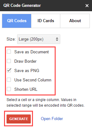
To create QR codes in Google Sheets, you first need to install a free add-on. To do that, select the option “Add-ons > Get add-ons.” Now, search for “QR Code Generator” and click on the button “Free” to install the add-on.

Once installed, select the data you want to create the QR code for and then select the option “Add-ons > QR Code Generator > Start.” Now, select the required options on the newly appeared sidebar and then click on the button “Generate” to create QR codes in Google Sheets.
5. Make Use of Templates
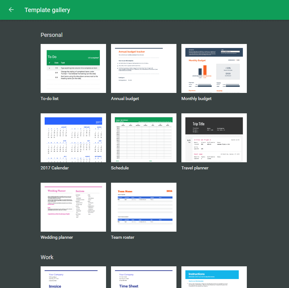
Depending on what type of Google spreadsheet you want to create, you don’t have to style it from ground up. Google Sheets has many templates to get you started with your next spreadsheet.
To access Google Sheets templates, create a new Google Sheet and then select the option “File > New > From template.” This action will open a new window where you can select the template of your choice.
6. Merge Cells
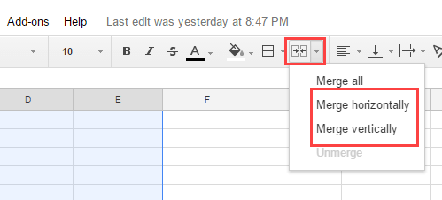
There will be times when you might want to merge cells so that you can add more data. To merge cells, select the cells you want to merge and then click on the “Merge” icon.
If you want to, you can also merge cells vertically or horizontally by selecting the option “Merge vertically” or “Merge Horizontally” respectively from the drop-down menu. To unmerge the merged cells and select the option “Unmerge.”
7. Add multiple Lines in a Single Cell
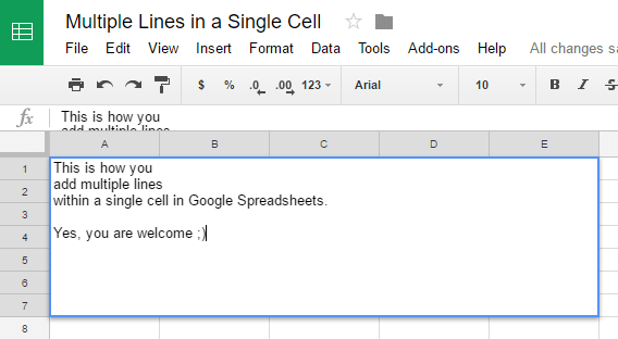
This Google Spreadsheet tip goes hand in hand with the merge cells tip we discussed above. When you merge cells, you might also want to add content in multiple lines. However, when you press the enter button, you will be moved to the next cell rather than the next line.
So, to add multiple lines in a single cell in Google Spreadsheets, all you have to do is press the keyboard shortcut Alt + Enter or Option + Return on Mac.
8. Make Use of The “Download As” Option
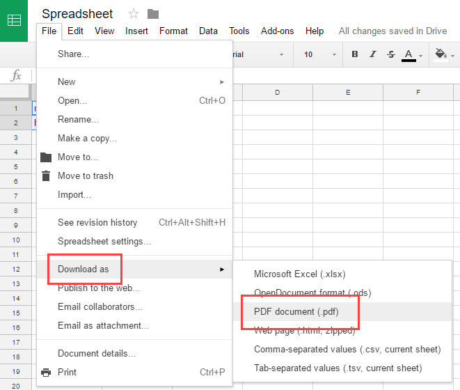
This is one of least know features of Google Sheets, but it is really useful when you want to download the Google Sheet in other formats. Using the “Download As” option you can download Google Sheets in different formats like PDF, XLSX, ODS, HTML, CSV, etc.
You can easily access this option by navigating “File > Download As“. Once you are here, select the appropriate format to download the Google Sheet.
9. Protect Ranges
If you are sharing your Google Sheet with others then it is only natural that you might want to protect some cells or a range of cells so that no one can change the data in those cells.
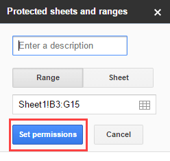
To protect a range, select the cells you want to protect and then select the option “Data > Protect Sheets and Ranges.” On the sidebar, click on the button “Set Permissions.”
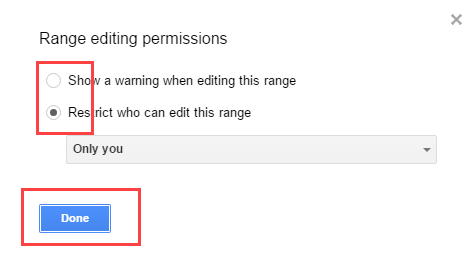
Now, select the appropriate editing permissions and then click on the button “Done.” That’s all there is to do and you are good to go.
———
Hope that helps and do comment below discussing how helpful these Google Spreadsheet tips are or to share your own favorite Google Spreadsheets tips.

